Quick tip: Publication worthy graphics with Mathematica

I am a huge fan of Mathematica for prototyping and quick one-offs. Most of the heavy lift analysis I do is with MATLAB or python, but sometimes I produce a graphic in Mathematica that I want to include in a publication. Here are a few tips on getting your Mathematica figures to look a little bit better.

I will use a sine wave with arbitrary labels as the example. A default labeled plot looks like this:

default = Plot[
  Sin[x],
  {x, 0, 2 \[Pi]},
  PlotLabel -> "Sine wave",
  AxesLabel -> {"Horiz. (unit)", "Vert. (unit)"}
]
Export["default.png", default]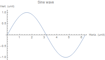

There are a few things I don’t like about this. First, the resolution is too low. Mathematica defaults to an image resolution of 72 dpi (dots per inch). Second, I want the text/axes to be black, not gray. Third, I think the labels for the axes should be to the left and below the figure, not at the positive ends of the axes. And finally, I would like for the horizontal axis to run along the bottom of the figure (and for the entire figure to be encapsulated in a frame).

Resolution

Both Plot and Export take the optional argument ImageSize. If we know the resolution of the image (which defaults to 72 dpi), we can use ImageSize to set the image to a specific width in inches. Here is the same figure resized to 3.2 inches (“ImageSize -> 3.2*72“):

res1 = Plot[
  Sin[x],
  {x, 0, 2 \[Pi]},
  PlotLabel -> "Sine wave",
  AxesLabel -> {"Horiz. (unit)", "Vert. (unit)"},
  ImageSize -> 3.2*72
]
Export["res1.png", res1]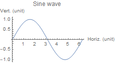

To increase the resolution of the image, we can use ImageResolution in Export. Plot does not take ImageResolution, so I tend to put ImageSize and ImageResolution in Export. This has the added benefit of not making the plots in Mathematica very large (since it still uses either 72 dpi or the screen dpi for display).

default = Plot[
  Sin[x],
  {x, 0, 2 \[Pi]},
  PlotLabel -> "Sine wave",
  AxesLabel -> {"Horiz. (unit)", "Vert. (unit)"}
]
Export["res2.png", default, ImageSize -> 3.2*300, 
 ImageResolution -> 300]

Well, that doesn’t look good! Unfortunately, there is a bug in how the PNG (and TIFF, and possibly other) exporters work. The axes/ticks don’t scale with image resolution. This is a known bug. One suggested solution is to export the plot as a PDF using ExportString and then immediately import it with ImportString. [Future me: The following may be the most important tip in this post.] I have found that including a PlotLegends will cause the scaling to work fine, even if the legend is not visible. I will typically do something like PlotLegends -> Placed["", {Right, Top}]. Using Placed makes the legend appear inside the frame, so that the width of the figure doesn’t change.

default2 = Plot[
  Sin[x],
  {x, 0, 2 \[Pi]},
  PlotLabel -> "Sine wave",
  AxesLabel -> {"Horiz. (unit)", "Vert. (unit)"},
  PlotLegends -> Placed["", {Right, Top}]
]
Export[res3.png", default2, ImageSize -> 3.2*300, 
 ImageResolution -> 300]

(Please note, that for these larger resolution images I am artificially restricting their display size to be the same as the original 72 dpi image, which I’ve increased to be close to 3.2 inches on my display. This is because I want them all to be 3.2 inches in print, but on a screen DPI doesn’t mean anything. In fact, I don’t even think PNG files keep track of DPI. When actually exporting for a journal/publication, I recommend using TIFF or EPS. With a vector format, you don’t even need to worry about all this ImageResolution nonsense. You can see the full resolution images by opening them in a new tab or saving them.)

Black text, labels, and frame

Thankfully, we can fix my remaining three complaints by turning off the axes and using a frame (Axes -> False and Frame -> True). I use BaseStyle to set the default font size for both the axes labels and the tick labels. FrameLabel sets the labels for all four sides of the frame in the order bottom, left, top, right. FrameStyle is used to set the frame to be black (which prints much better than the default gray).

frame =
 Plot[
  Sin[x],
  {x, 0, 2 \[Pi]},
  BaseStyle -> {FontSize -> 12},
  PlotLegends -> Placed["", {Left, Top}],
  FrameLabel -> {"Horiz. (unit)", "Vert. (unit)", 
    Style["Sine wave", 16], None},
  Axes -> False,
  Frame -> True,
  FrameStyle -> Black
]
Export["frame1.png", frame, ImageSize -> 3.2*300, 
 ImageResolution -> 300]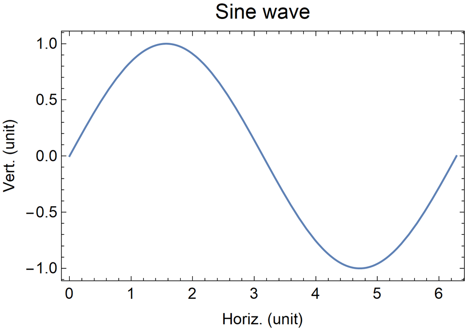

Bonus: Legends and color

I mentioned needing to use PlotLegends to get around a scaling bug. I also talked about Placed, but I’d like to say a bit more about that. By default, Mathematica places the legends outside of the frame. In most cases, this is not desirable. You can place the legends inside the frame with Placed[legends, {horiz. pos., vert. pos.}]. I used to get confused if I should say {Top, Right} or {Right, Top} until I realized the first was for horizontal positioning and the second was for vertical positioning. Also, please don’t use the default Mathematica colors in print.

frame2 =
 Plot[
  {Sin[x], Cos[x]},
  {x, 0, 2 \[Pi]},
  PlotStyle -> {Blue, Red},
  BaseStyle -> {FontSize -> 12},
  PlotLegends -> Placed[{"Sine", "Cosine"}, {Left, Bottom}],
  FrameLabel -> {"Horiz. (unit)", "Vert. (unit)"},
  Axes -> False,
  Frame -> True,
  FrameStyle -> Black
]
Export["frame2.png", frame2, ImageSize -> 3.2*300, 
 ImageResolution -> 300]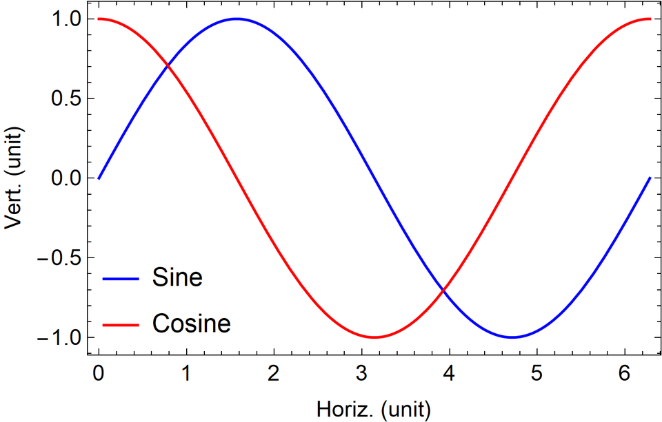

Do you have any Mathematica tips for making better figures? Please share them in a comment to this post. Thanks for reading!